Flowmetering

Introduction

Many industrial and commercial businesses have now recognised the value of:

• Energy cost accounting.
• Energy conservation.
• Monitoring and targeting techniques.

These tools enable greater energy efficiency.

Steam is not the easiest media to measure. The objective of this Block is to achieve a greater understanding of the requirements to enable the accurate and reliable measurement of steam flowrate.

Most flowmeters currently available to measure the flow of steam have been designed for measuring the flow of various liquids and gases. Very few have been developed specifically for measuring the flow of steam.

Spirax Sarco wishes to thank the EEBPP (Energy Efficiency Best Practice Programme) of ETSU for contributing to some parts of this Block..

Why measure steam?

Steam flowmeters cannot be evaluated in the same way as other items of energy saving equipment or energy saving schemes. The steam flowmeter is an essential tool for good steam housekeeping. It provides the knowledge of steam usage and cost which is vital to an efficiently operated plant or building. The main benefits for using steam flowmetering include:

• Plant efficiency.
• Energy efficiency.
• Process control.
• Costing and custody.

Plant efficiency

 A good steam flowmeter will indicate the flowrate of steam to a plant item over the full range of its operation, i.e. from when machinery is switched off to when plant is loaded to capacity. By analysing the relationship between steam flow and production, optimum working practices can be determined.

The flowmeter will also show the deterioration of plant over time, allowing optimum plant cleaning or replacement to be carried out.

The flowmeter may also be used to:

This may lead to changes in production methods to ensure economical steam usage. It can also reduce problems associated with peak loads on the boiler plant.

Energy efficiency

Steam flowmeters can be used to monitor the results of energy saving schemes and to compare the efficiency of one piece of plant with another.

Process control

The output signal from a proper steam flowmetering system can be used to control the quantity of steam being supplied to a process, and indicate that it is at the correct temperature and pressure.

Also, by monitoring the rate of increase of flow at start-up, a steam flowmeter can be used in conjunction with a control valve to provide a slow warm-up function.

Costing and custody

Steam flowmeters can measure steam usage (and thus steam cost) either centrally or at individual user points. Steam can be costed as a raw material at various stages of the production process thus allowing the true cost of individual product lines to be calculated.

To understand flowmetering, it might be useful to delve into some basic theory on fluid mechanics, the characteristics of the fluid to be metered, and the way in which it travels through pipework systems.

Fluid characteristics

Every fluid has a unique set of characteristics, including:

• Density.
• Dynamic viscosity
• Kinematic viscosity.

Density

This has already been discussed in Block 2, Steam Engineering Principles and Heat Transfer, however, because of its importance, relevant points are repeated here.

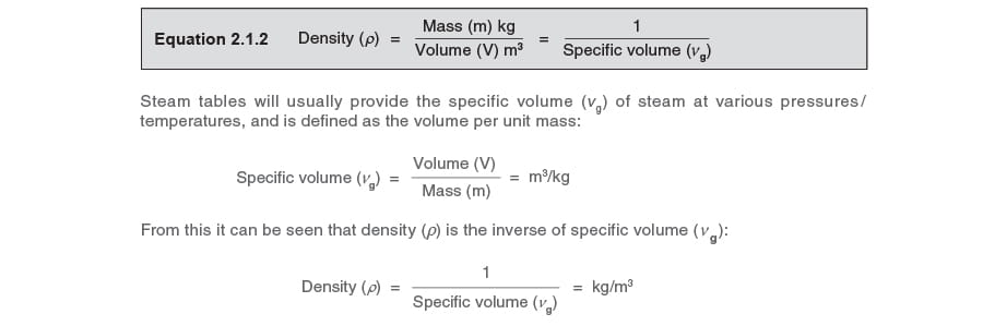
Density (ρ) defines the mass (m) per unit volume (V) of a substance (see Equation 2.1.2).

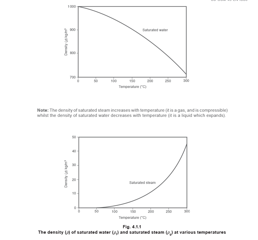
The density of both saturated water and saturated steam vary with temperature. This is illustrated in Figure 4.1.1.

Dynamic viscosity

This is the internal property that a fluid possesses which resists flow. If a fluid has a high viscosity (e.g. heavy oil) it strongly resists flow. Also, a highly viscous fluid will require more energy to push it through a pipe than a fluid with a low viscosity.

There are a number of ways of measuring viscosity, including attaching a torque wrench to a paddle and twisting it in the fluid, or measuring how quickly a fluid pours through an orifice.

A simple school laboratory experiment clearly demonstrates viscosity and the units used:

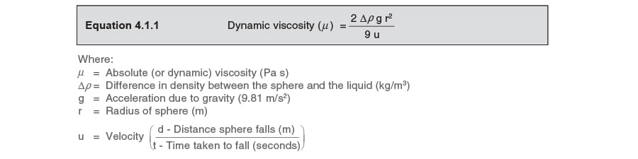
A sphere is allowed to fall through a fluid under the influence of gravity. The measurement of the distance (d) through which the sphere falls, and the time (t) taken to fall, are used to determine the velocity (u).

The following equation is then used to determine the dynamic viscosity:

There are three important notes to make:

1. The result of Equation 4.1.1 is termed the absolute or dynamic viscosity of the fluid and is measured in pascal seconds. Dynamic viscosity is also expressed as ‘viscous force.’

2. The physical elements of the equation give a resultant in kg/m, however, the constants (2 and 9) take into account both experimental data and the conversion of units to pascal seconds (Pa s).

3. Some publications give values for absolute viscosity or dynamic viscosity in centipoise (cP), e.g.: 1 cP = 10-3 Pa s

Example 4.1.1

It takes 0.7 seconds for a 20mm diameter steel (density 7 800 kg/m3) ball to fall 1 metre through oil at 20°C (density = 920 kg/m3).

Kinematic viscosity
This expresses the relationship between absolute (or dynamic) viscosity and the density of the fluid (see Equation 4.1.2).

Example 4.1.2

In Example 4.1.1, the density of the oil is given to be 920 kg/m3 - Now determine the kinematic viscosity:

Reynolds number (R_e)

The factors introduced above all have an effect on fluid flow in pipes. They are all drawn together in one dimensionless quantity to express the characteristics of flow, i.e. the Reynolds number (R_e).

Analysis of the equation will show that all the units cancel, and Reynolds number (R_e) is therefore dimensionless.

Evaluating the Reynolds relationship:
• For a particular fluid, if the velocity is low, the resultant Reynolds number is low
• If another fluid with a similar density, but with a higher dynamic viscosity is transported through the same pipe at the same velocity, the Reynolds number is reduced
• For a given system where the pipe size, the dynamic viscosity (and by implication, temperature) remain constant, the Reynolds number is directly proportional to velocity

Example 4.1.3
The fluid used in Examples 4.1.1 and 4.1.2 is pumped at 20 m/s through a 100 mm bore pipe.

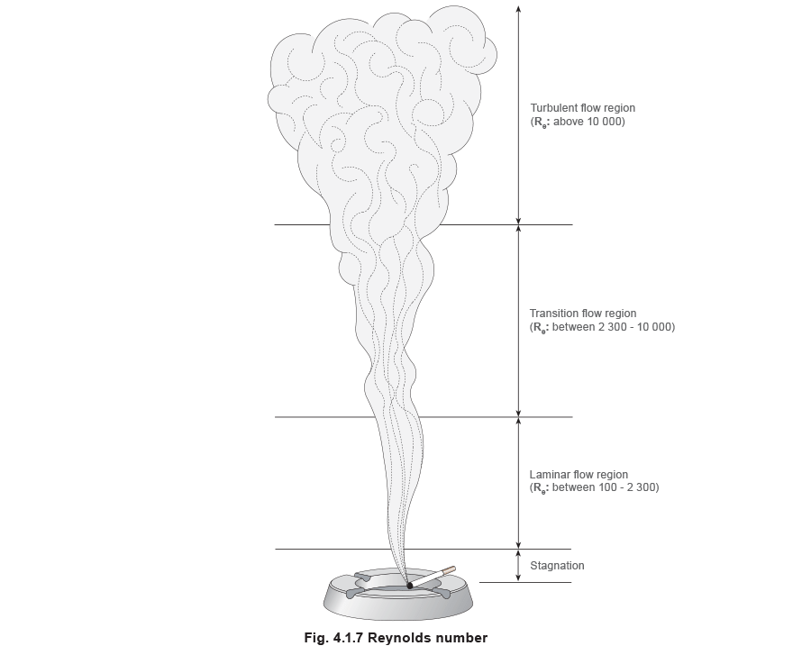
From looking at the above Reynolds number it can be seen that the flow is in the laminar region (see Figure 4.1.7).

 Flow regimes

If the effects of viscosity and pipe friction are ignored, a fluid would travel through a pipe in a uniform velocity across the diameter of the pipe. The ‘velocity profile’ would appear as shown in Figure 4.1.3:

However, this is very much an ideal case and, in practice, viscosity affects the flowrate of the fluid and works together with the pipe friction to further decrease the flowrate of the fluid near the pipe wall. This is clearly illustrated in Figure 4.1.4:

At low Reynolds numbers (2 300 and below) flow is termed ‘laminar’, that is, all motion occurs along the axis of the pipe. Under these conditions the friction of the fluid against the pipe wall means that the highest fluid velocity will occur at the centre of the pipe (see Figure 4.1.5).

As the velocity increases, and the Reynolds number exceeds 2 300, the flow becomes increasingly turbulent with more and more eddy currents, until at Reynolds number 10 000 the flow is completely turbulent (see Figure 4.1.6).

Saturated steam, in common with most fluids, is transported through pipes in the ‘turbulent flow’ region.

The examples shown in Figures 4.1.3 to 4.1.7 are useful in that they provide an understanding of fluid characteristics within pipes; however, the objective of the Steam and Condensate Loop Book is to provide specific information regarding saturated steam and water (or condensate).
Whilst these are two phases of the same fluid, their characteristics are entirely different. This has been demonstrated in the above Sections regarding Absolute Viscosity and Density. The following information, therefore, is specifically relevant to saturated steam systems.

Example 4.1.4
A 100 mm pipework system transports saturated steam at 10 bar g at an average velocity of 25 m/s.
Determine the Reynolds number. The following data is available from comprehensive steam tables:

• If the Reynolds number (R_e) in a saturated steam system is less than 10 000 (104) the flow may be laminar or transitional.
Under laminar flow conditions, the pressure drop is directly proportional to flowrate.
• If the Reynolds number (R_e) is greater than 10 000 (104) the flow regime is turbulent.
Under these conditions the pressure drop is proportional to the square root of the flow.
• For accurate steam flowmetering, consistent conditions are essential, and for saturated steam systems it is usual to specify the minimum Reynolds number (R_e) as 1 x 105 = 100 000.
• At the opposite end of the scale, when the Reynolds number (R_e) exceeds 1 x 106, the head losses due to friction within the pipework become significant, and this is specified as the maximum.

Example 4.1.5
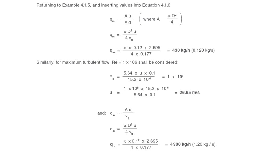
Based on the information given above, determine the maximum and minimum flowrates for turbulent flow with saturated steam at 10 bar g in a 100 mm bore pipeline.

Returning to Example 4.1.5, and inserting values into Equation 4.1.6:

Summary
• The mass flow of saturated steam through pipes is a function of density, viscosity and velocity.
• For accurate steam flowmetering, the pipe size selected should result in Reynolds numbers of between 1 x 105 and 1 x 106 at minimum and maximum conditions respectively.
• Since viscosity, etc., are fixed values for any one condition being considered, the correct Reynolds number is achieved by careful selection of the pipe size.
• If the Reynolds number increases by a factor of 10 (1 x 105 becomes 1 x 106), then so does the velocity (e.g. 2.695 m/s becomes 26.95 m/s respectively), providing pressure, density and viscosity remain constant.